
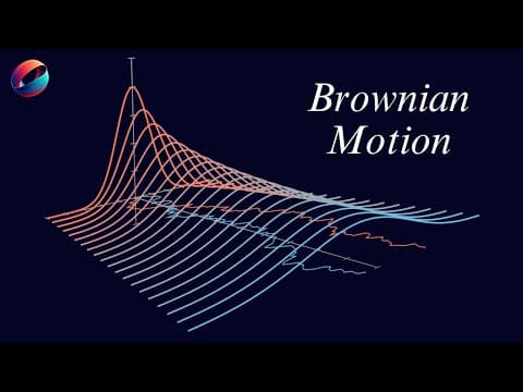
This blog post explores Brownian motion, a fundamental stochastic process in finance, detailing its definition, properties, and significance in modeling stock prices through geometric Brownian motion.
In the realm of stochastic calculus, Brownian motion stands out as a unique and fundamental stochastic process. This blog post aims to provide a comprehensive understanding of Brownian motion, its origins, properties, and its application in modeling financial markets.
Brownian motion can be thought of as a continuous-time stochastic process that is essential for modeling various phenomena in finance. To grasp its concept, we can start by examining a simpler process known as a random walk.
A random walk can be illustrated through a coin-flipping experiment. Each flip results in either heads or tails, which correspond to upward or downward movements in a hypothetical stock price. Mathematically, we can define a random variable associated with this event, denoted as X_i, where the expectation of X_i is zero and the variance is one. The cumulative sum of these movements can be represented as Y_n, which reflects the stock price.
However, a basic random walk is discrete, meaning it only takes values at specific points (0, 1, 2, 3, etc.). This limitation makes it unsuitable for modeling continuous financial markets where prices fluctuate every second.
To address the limitations of the basic random walk, we can introduce the concept of a scaled random walk. By increasing the frequency of coin flips, we can obtain values at smaller intervals (e.g., 0, 0.5, 1, 1.5, etc.). As we continue to scale down the intervals, the resulting paths begin to resemble the continuous fluctuations observed in stock prices.
Brownian motion can be formally defined with several key properties:
As time progresses, the variance increases, indicating that the Brownian motion spreads further from the origin.
Several important properties characterize Brownian motion:
These properties highlight the erratic and unpredictable nature of Brownian motion, making it a crucial concept in stochastic calculus.
Quadratic variation is a significant aspect of Brownian motion. Unlike total variation, which sums absolute differences, quadratic variation squares these differences. For differentiable functions, the quadratic variation equals zero. However, for Brownian motion, it is non-zero due to its unpredictable nature. This property is essential for understanding the behavior of financial instruments modeled by Brownian motion.
To model stock prices more accurately, we introduce geometric Brownian motion. This model accounts for the proportional changes in stock prices based on their current value. For instance, a stock priced at $10,000 will experience larger absolute changes than a stock priced at $100, even if both have the same percentage change.
Geometric Brownian motion incorporates two critical components:
The differential equation governing geometric Brownian motion allows for simulations and provides a more realistic model for stock price behavior.
Brownian motion is a foundational concept in stochastic calculus, particularly in quantitative finance. Its properties and the introduction of geometric Brownian motion enable more accurate modeling of stock prices, reflecting the complexities of financial markets. Understanding these concepts is crucial for anyone looking to delve into the world of finance and stochastic processes.