This blog post explains the concept of SOFR futures, their mechanics, and how they can be used as a hedging instrument in financial transactions, illustrated through a practical example involving a $100 million borrowing.
In this blog post, we will explore the concept of SOFR futures, how they operate, and their practical applications in financial transactions. We will break down the mechanics of these futures contracts and illustrate their use through a straightforward example.
SOFR stands for the Secured Overnight Financing Rate. It is a benchmark interest rate designed to replace the USD LIBOR (London Interbank Offered Rate). SOFR represents the interest cost on overnight borrowing that is collateralized by U.S. Treasuries.
SOFR futures are futures contracts that reference SOFR. These contracts are traded on the Chicago Mercantile Exchange (CME). They allow market participants to hedge against fluctuations in interest rates.
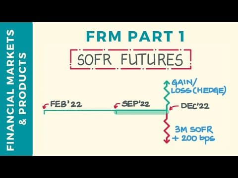
To understand how SOFR futures work, let’s consider a practical example involving a $100 million borrowing.
The three-month SOFR is derived from the daily observed SOFR rates during the borrowing period. These daily rates are compounded to arrive at the three-month implied SOFR for the entire period. The observation period runs from September 21 to December 20, 2022.
As the borrowing date approaches, there is a risk that interest rates may rise, leading to increased borrowing costs. To mitigate this risk, the borrower can use SOFR futures as a hedging instrument.
There are two types of SOFR futures available on the CME:
For our example, we will use the three-month SOFR futures, which are designed to be structurally similar to Eurodollar futures contracts.
If the implied three-month SOFR changes by one basis point (0.01%), the gain or loss for one three-month SOFR futures contract is $25. This is calculated as follows:
[ \text{Gain/Loss} = 0.01 \times 1,000,000 \times 0.25 = 25 \text{ dollars} ]
Assuming the three-month SOFR futures are trading at 98.495, the implied three-month SOFR is:
[ 100 - 98.495 = 1.505% ]
To hedge against rising interest rates, the borrower should take a short position in the September 2022 three-month SOFR futures. Given the borrowing amount of $100 million and the notional amount of $1 million per contract, the borrower will need:
[ \text{Number of Contracts} = \frac{100,000,000}{1,000,000} = 100 \text{ contracts} ]
On December 20, 2022, if the final settlement price for the SOFR futures is 98.2, the implied three-month SOFR becomes:
[ 100 - 98.2 = 1.8% ]
The interest cost on the borrowing will be:
[ 100,000,000 \times 1.8% + 2% \text{ fixed spread} \times 0.25 = 950,000 \text{ dollars} ]
Simultaneously, the gain or loss from the SOFR futures hedge can be calculated. The change in the futures price from 98.495 to 98.2 results in a gain:
[ \text{Gain} = 100 \times (98.495 - 98.2) \times 2500 = 73,750 \text{ dollars} ]
The net interest cost after accounting for the hedge gain is:
[ 950,000 - 73,750 = 876,250 \text{ dollars} ]
This demonstrates how the borrower effectively locked in a value of the three-month implied SOFR at 1.505% through the use of SOFR futures.
In summary, SOFR futures provide a valuable tool for managing interest rate risk in financial transactions. By understanding their mechanics and applying them in practical scenarios, borrowers can effectively hedge against potential increases in interest rates, ensuring more predictable borrowing costs. This example illustrates the importance of SOFR futures in modern finance and their role in risk management strategies.