
This blog post explores the different types of spatial data, their analysis techniques, and common pitfalls in spatial analysis, emphasizing the importance of data structure and appropriate methodologies for accurate conclusions.
Spatial data analysis is a crucial aspect of understanding geographic features and their relationships. This post delves into the various types of spatial data, the analytical techniques associated with them, and the common pitfalls that researchers should be aware of when conducting spatial analysis.
Spatial data can be categorized into formal representations of geographic features, often referred to as data structures in spatial analysis. The primary types of spatial data include:
Points are the simplest form of spatial data, represented by x and y coordinates. They can denote fixed locations, such as addresses of houses, or random events, such as the locations of accidents or crimes. Analyzing point data often involves examining point patterns to determine if there is any structure or clustering in the distribution of these events. For instance, a heat map can illustrate concentrations of car thefts in a city, helping to identify areas with higher crime rates.
Surfaces represent continuous spatial fields, such as air quality or temperature. Unlike discrete points, surfaces approximate phenomena that vary continuously across a geographic area. The analysis of surfaces often involves interpolation, which predicts values for locations where direct measurements are not available. For example, researchers may use sensor data to estimate air quality across a region, linking it to housing prices to understand economic implications.
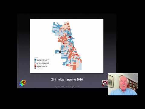
Lattice data consists of aerial units, such as census tracts or counties, represented as polygons. The analysis of lattice data focuses on locational and attribute similarities, allowing researchers to identify patterns such as hot spots or cold spots. For example, a map showing income inequality across census tracts can reveal areas of high and low inequality, facilitating targeted policy interventions.
The type of spatial data dictates the analytical techniques employed. Here are some common methods:
While spatial analysis can yield valuable insights, researchers must be cautious of several pitfalls:
This occurs when individual behaviors are inferred from aggregate data. For example, using county-level crime data to explain individual criminal behavior can lead to misleading conclusions. It is essential to match the scale of the analysis with the scale of the data.
MAUP refers to the issues arising from the choice of spatial units for analysis. The results can vary significantly depending on how data is aggregated, which can lead to conflicting interpretations. Researchers must carefully consider the appropriate scale and arrangement of spatial units.
COSP arises when variables are measured at different spatial scales, complicating the analysis. For instance, school districts may not align neatly with census data, making it challenging to derive meaningful statistics. Solutions often involve aggregating data to a common scale or using advanced statistical methods like Bayesian statistics.
Understanding the types of spatial data and the associated analytical techniques is vital for conducting effective spatial analysis. Researchers must remain vigilant about common pitfalls, ensuring that their methodologies align with the data structures they are working with. By doing so, they can draw accurate conclusions and contribute valuable insights to their fields of study.
As you embark on your spatial analysis projects, take the time to reflect on these concepts and their implications for your work. If you have questions or need further clarification, don't hesitate to reach out for assistance.