
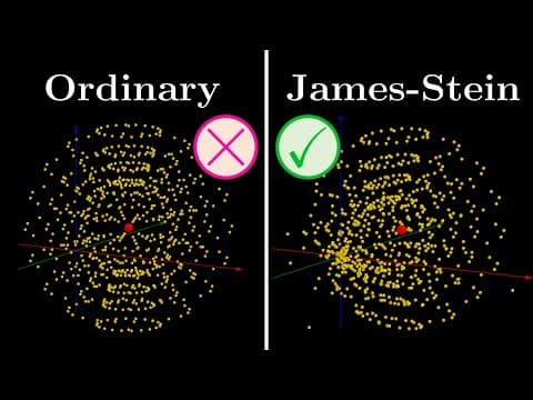
Stein's paradox reveals that the James-Stein estimator outperforms traditional maximum likelihood estimation in estimating means from multiple independent normal distributions, highlighting the importance of shrinkage and the bias-variance tradeoff in statistics and machine learning.
In 1961, a groundbreaking paper divided the statistics community by challenging the long-held beliefs of influential statistician Ronald Fisher regarding maximum likelihood estimation. This paper introduced what is now known as Stein's paradox, a concept that has profound implications in statistics and machine learning. This article explores the essence of Stein's paradox, the mechanics of the James-Stein estimator, and the broader lessons it teaches about estimation.
To understand Stein's paradox, we start with a simple scenario. Imagine we have a set of data that follows a normal distribution with an unknown mean (mu) and a variance of 1. If we randomly select a data point from this distribution, say 3.14, a reasonable estimate for mu would be 3.14 itself. This is considered the best estimator in this context because it is the most sensible guess based on the available information.
Now, consider two independent sets of data, both following normal distributions with means mu_1 and mu_2. If we select data points 3.14 and 1.618 from these distributions, we would again estimate mu_1 as 3.14 and mu_2 as 1.618. This method remains the best estimator in this case.
However, the situation changes dramatically when we introduce a third independent set of data. In this case, the ordinary estimator—simply echoing back the data points—no longer holds as the best method. Instead, the James-Stein estimator emerges as a superior alternative. This estimator incorporates all three data points to provide a more accurate estimate for mu_1, which is surprising given that the data sets are independent.
The James-Stein estimator generalizes to p sets of data (where p is at least 3) and consistently outperforms the ordinary estimator in higher dimensions. This revelation caused significant upheaval in the statistics community, as it contradicted the well-established theory of maximum likelihood estimation, which suggested that the best approach was to rely solely on the data points provided.
To determine what makes an estimator the "best," we use the mean squared error (MSE). The MSE quantifies the average squared difference between the estimated value (mu hat) and the true mean (mu). In the case of multiple data sets, we treat the estimators as vectors and calculate the squared error for each component, summing them up and averaging the results. This process accounts for the randomness inherent in the estimator.
For example, in a one-dimensional case, the ordinary estimator's MSE is constant at 1, while a naive estimator that always guesses 7 has a MSE that varies depending on the true mean mu. This leads to the concept of dominance: if one estimator consistently has a lower MSE than another, it is said to dominate that estimator.
The James-Stein estimator introduces a shrinkage factor that adjusts the estimates based on the data points. This factor typically ranges between 0 and 1, but can become negative if the data points are too small. Despite this potential flaw, the James-Stein estimator still outperforms the ordinary estimator.
Geometrically, we can visualize the true means as points in a multi-dimensional space. The shrinkage factor minimizes the average distance from these points to the true mean. While it may increase the distance for points already close to the origin, it significantly reduces the distance for points further away, leading to an overall reduction in error.
A critical concept illustrated by the James-Stein estimator is the bias-variance tradeoff. The mean squared error can be decomposed into two components: variance and bias. An estimator with low bias may have high variance, leading to larger errors, while introducing a small bias can reduce variance significantly, resulting in a lower overall mean squared error.
In modern statistics and machine learning, the lessons from Stein's paradox are invaluable. When dealing with complex models that require estimating multiple parameters, the shrinkage effect can dramatically reduce mean squared error, especially as the number of parameters increases. This principle is foundational in regularization techniques used in machine learning, where the goal is to improve model performance by reducing overfitting.
Stein's paradox and the James-Stein estimator challenge traditional notions of estimation in statistics. By demonstrating that incorporating information from multiple independent data sets can lead to better estimates, these concepts underscore the importance of understanding the bias-variance tradeoff and the role of shrinkage in modern statistical practices. As we continue to navigate increasingly complex data landscapes, the insights gained from Stein's paradox will remain relevant and essential for effective statistical modeling and machine learning.